A Markov chain containing absorbing states is known as an absorbing Markov chain. So what is an absorbing state. In simple words, if you end up on an absorbing state you can’t go anywhere else; you are stuck there for all eternity. In other words, the probability of transition from an absorbing state $i$ to any other non-absorbing state, also called transient states, is 0.
At this point, we can make an observation:
0. The probability of eventually begin absorbed into any of the absorbing states given that one starts from anywhere is 1.
Let’s say we have $n$ transient states and $m$ absorbing states in the state space of any system. The transition matrix for such a system can be written as:
$$T = \left[ \begin{matrix} Q & R \\ 0 & I \end{matrix} \right],$$
where $Q$ of shape ($n \times n$) gives the probability of transitioning from transient state $i$ to transient state $j$. The matrix $R$ of shape $n \times m$ gives the probability of transitioning from transient state $i$ to absorbing state $j$, and $I$ of identity matrix of shape $m$.
We can compute the respective probability weights of the various states given a current probability weights by applying the transition matrix following the Markov property:
\[v_{k+1} = T\ v_{k}\]Recursively expanding the above equation to the starting state $v_0$, we have
\[v_{k} = T^k\ v_{0}\]It is interesting to compute what $T^k$ is:
$$ \begin{align} T^2 &= \begin{bmatrix} Q & R \\ 0 & I \end{bmatrix} \begin{bmatrix} Q & R \\ 0 & I \end{bmatrix} = \begin{bmatrix} Q^2 & QR + RI \\ 0 & I \end{bmatrix} \\ T^3 &= \begin{bmatrix} Q & R \\ 0 & I \end{bmatrix} \begin{bmatrix} Q^2 & QR + RI \\ 0 & I \end{bmatrix} = \begin{bmatrix} Q^3 & Q^2R + QR + RI \\ 0 & I \end{bmatrix} \end{align} $$
Given the pattern we can write
$$T^k = \begin{bmatrix} Q^k & R(I + Q + Q^2 + ... + Q^k) \\ 0 & I \end{bmatrix}$$
Using the summation formula for a geometric sequence we can write:
$$ T^k = \begin{bmatrix} Q^k & R \left(\frac{I - Q^k}{I - Q}\right) \\ 0 & I \end{bmatrix} $$
From the above formula, we note that:
1. the probability the system is in transient state $j$ given that it started in transient state $i$ after $k$ steps is given by the $(i, j)^{th}$ entry of the matrix $Q^k$
The entries of $Q$ are all smaller than 1, given that these are probabilities. Hence we have $\lim_{k \to \infty} Q^k = 0$. This allows us to write
$$T^\infty = \begin{bmatrix} 0 & R \left(\frac{1}{I - Q}\right) \\ 0 & I \end{bmatrix} = \begin{bmatrix} 0 & NR \\ 0 & I \end{bmatrix},$$
where $N = [I - Q]^{-1}$ is known as the fundamental matrix. The $0’s$ in the first column of the above matrix proves statement given in blockquote 0.
From the above formula, we note that:
2. the probability the system ends up in absorbing state $j$ given that it started in transient state $i$ is the $(i, j)^{th}$ entry of the matrix $NR$.
The fundamental matrix $N$ has a very interesting interpretation:
3. its $(i, j)^{th}$ entry corresponds to the expected number of times the system visits transient state $j$ given that it started in transient state $i$, before being absorbed.
To see this, let us use a random indicator variable $\mathcal{I}_k$ which is 1 if the system is in state $j$ during $k^{th}$ step, else 0. The expected value of this indicator variable is:
\[E[\mathcal{I}_k] = 1 \times prob(\mathcal{I}_k = 1) + 0 \times prob(\mathcal{I}_k = 1) = Q^k_{i, j} \quad ......... \text{refer blockquote 1}\]The total number of visits we make to state $j$ in $n$ steps of the Markov chain is simply summing up all these indicator variables (one for each step).
\[\text{total_visits after $n$ steps} = \mathcal{I}_0 + \mathcal{I}_1 + \mathcal{I}_2 + .....+\ \mathcal{I}_n\]Taking the expectation we get
$$ \begin{align} E[\text{total_visits after $n$ steps}] &= E[\mathcal{I}_0] + E[\mathcal{I}_1] + E[\mathcal{I}_2] + .....+\ E[\mathcal{I}_n] \\ &= Q^0_{i, j} +\ Q^1_{i, j} +\ ...+\ Q^n_{i, j} \end{align} $$
Taking $n \to \infty$, we have \(E[\text{total_visits}] = Q^0_{i, j} +\ Q^1_{i, j} +\ ...+\ Q^\infty_{i, j} = [I - Q]^{-1}_{i, j} = N_{i, j}\)
Summing this over all the possible transient states, we get the expected number of steps the Markov chain runs for, starting at state $i$, before getting absorbed into one of the absorbing states. This is nothing but adding the entries of the $i^{th}$ row of $N_{i, j}$:
\[t_i = \sum_j N_{i, j}\]Q1. On average, how many times do we have to roll a fair dice before seeing two 6’s in a row?
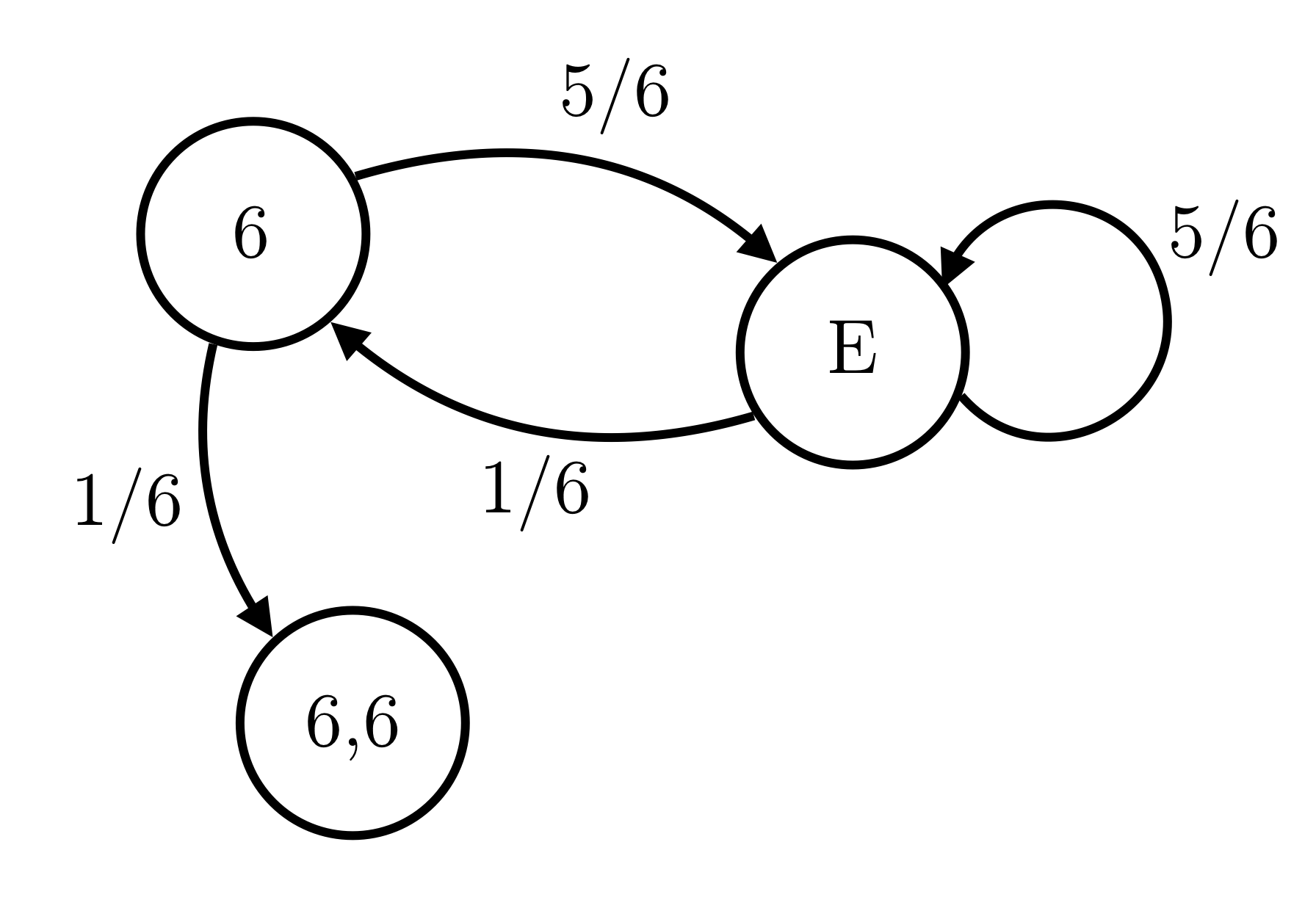
Solution: One can represent the state space as $S = [6, E, 66]$, with $66$ being the absorbing state.

where $E = \{\phi, 1, 2, 3, 4, 5\}$. $\phi$ represents the null state $\to$ the state before we even began rolling the dice.
The transition matrix can be written as:
$$T = \begin{bmatrix} 0 & 5/6 & 1/6 \\ 1/6 & 5/6 & 0 \\ 0 & 0 & 1\end{bmatrix},$$
where the labels corresponds to the index as given in $S$. The fundamental matrix $N$ is given by:
$$ \begin{align} N = [I - Q]^{-1} &= \left(\begin{bmatrix} 1 & 0 \\ 0 & 1 \end{bmatrix} - \begin{bmatrix} 0 & 5/6 \\ 1/6 & 5/6 \end{bmatrix}\right)^{-1}\\ &= \begin{bmatrix} 6 & 30 \\ 6 & 36 \end{bmatrix} \end{align} $$
Since we begin in state $\phi$ which is at index $1$ (assuming 0 indexing), the average number of dice rolls before seeing two 6’s in a row is
\[t_1 = N_{1,0} + N_{1, 1} = 42\]Q2. You keep on tossing a fair coin until you see HHT or THT. Which of these combination is more likely to occur?
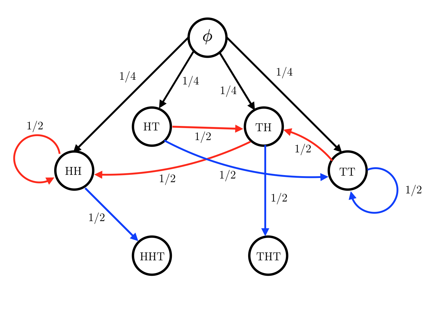
The trick in most of such problems is to correctly identify the relevant state space. For this problem, the state space that we can use is $S = [\phi, HH, HT, TH, TT, HHT, THT]$, where $HHT$ and $THT$ are the absorbing state. The transition diagram then becomes:

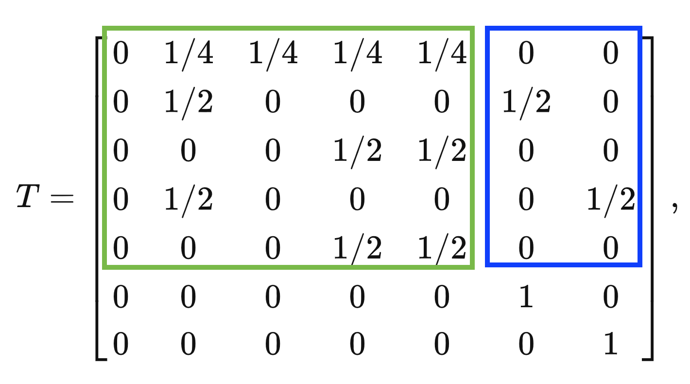
The red arrows indicates rolling a heads on the next roll, while blue arrows indicate rolling a tails on the next turn. Given this, the transition matrix becomes:

where the labels corresponds to the index as given in $S$. The fundamental matrix then becomes:
$$N = [I - Q]^{-1} = \begin{bmatrix} 1 & 0 & 0 & 0 & 0 \\ 0 & 1 & 0 & 0 & 0 \\ 0 & 0 & 1 & 0 & 0\\ 0 & 0 & 0 & 1 & 0\\ 0 & 0 & 0 & 0 & 1\\ \end{bmatrix}, $$
where the $Q$ matrix is shown in green box. Following blockquote 2. the required matrix is given by:
$$P = NR = \begin{bmatrix} 5/8 & 3/8 \\ 1 & 0 \\ 1/2 & 1/2 \\ 1/2 & 1/2 \\1/2 & 1/2 \end{bmatrix},$$
where $R$ is the matrix shown in blue. Thus the probability of starting from $\phi$ and ending up in the $HHT$ state is $5/8$, while ending up in the $THT$ state is $3/8$.
Q3. On average, how many times must a 6-sided die be rolled until all sides appear at least once? What about for an n-sided die?
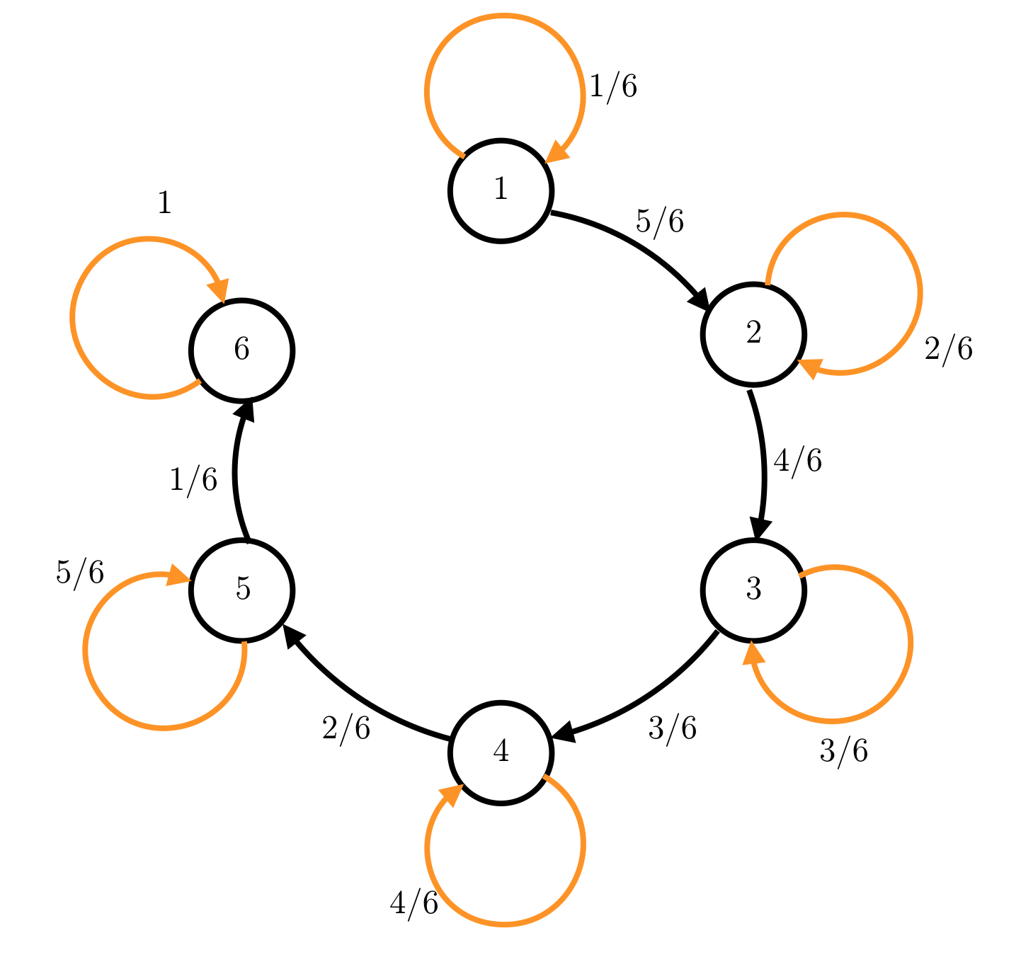
Let $n_i$ be the number of times face $i$ has shown up since we started rolling the dice. We now define an indicator variable $\mathcal{I}_i = \mathcal{I} (n_i > 0)$ and a random variable $X$ that is the sum of these indicator variables $\mathcal{I}_1$ to $\mathcal{I}_6$. The possible values of $X$ serves as the states of the system, i.e. $S = [1, 2, 3, 4, 5, 6]$.
The state $X=6$ can then be identified as the absorbing state, which happens when we see all the faces of the dice. The state diagram is given as:

The transition matrix corresponding to this can be written as:
$$T = \begin{bmatrix} 1/6 & 5/6 & 0 & 0 & 0 &0 \\ 0 & 2/6 & 4/6 & 0 & 0 &0\\ 0 & 0 & 3/6 & 3/6 & 0 &0\\ 0 & 0 & 0 & 4/6 & 2/6 &0\\ 0 & 0 & 0 & 0 & 5/6 &1/6\\ 0 & 0 & 0 & 0 & 0 & 1 \end{bmatrix},$$
where the labels corresponds to the index as given in $S$. The fundamental matrix is given by:
$$N = [I - Q]^{-1} = \begin{bmatrix} 1.2 & 1.5 & 2 & 3 & 6 \\ 0 & 1.5 & 2 & 3 & 6\\ 0 & 0 & 2 & 3 & 6\\ 0 & 0 & 0 & 3 & 6\\ 0 & 0 & 0 & 0 & 6 \end{bmatrix}$$
Since we begin in state $1$ (after one dice roll) which is at index $0$, the average number of dice rolls before seeing all sides appear is:
\[t_{\phi} = 1 + \sum_{j} N_{0j} = 1 + (1.2 + 1.5 + 2 + 3 + 6) = 14.7\]The $1$ in the above equation is needed since initially we start with no dice roll (state $\phi$). The above summation can be written in an interesting way:
\[t_{\phi} = 6\left(\frac{1}{6} + \frac{1}{5} + \frac{1}{4} + \frac{1}{3} + \frac{1}{2} + 1 \right)\]The quantity in the bracket is nothing but the $6^{th}$ Harmonic number $H_6$. Hence generalizing to arbitrary sided dice, the expected number of rolls required before seeing all the faces of the $n-sided$ dice is:
\[t_n = n\ H_n\]