Let’s imagine rain falling. One obvious parameter describing this process is the rate - whether its drizzling or pouring! Let’s now focus on a tiny patch of land and assume that the rate is constant and will term this as $\lambda$. We can describe rain as a Poisson process.
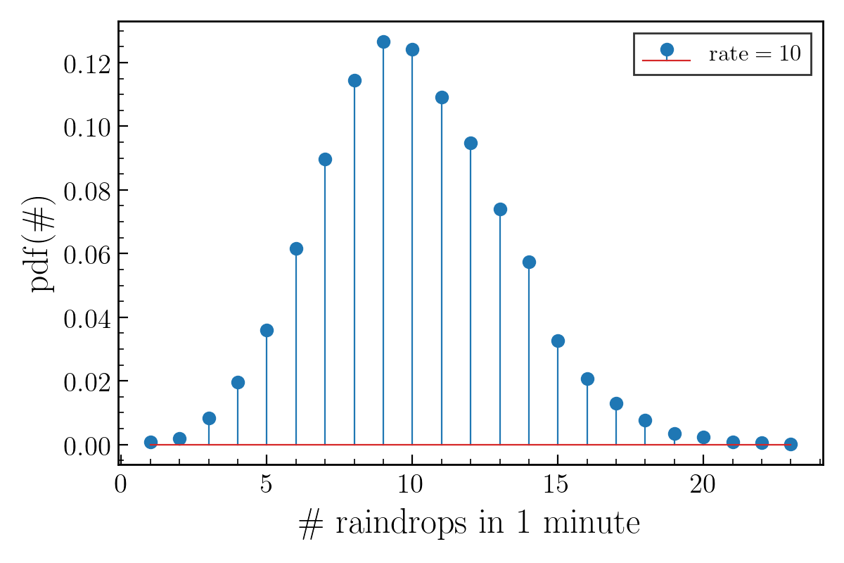
Now what in the world is a Poisson process. If we think $\lambda$ as the number of raindrops falling on the patch per minute, and let’s say we wait for 5 minutes; how many raindrops will we see? Well, on average we would see $5\lambda$ drops. However, we might see more or we might see less. A Poisson process is one in which this count of drops is Poisson distributed.
This discrete probability distribution is given by:
\[P(k\ \mathrm{events\ in\ interval}\ t) = \frac{ (\lambda t)^k e^{-\lambda t}}{k!}\]

An interesting property about Poisson distribution is that its mean and variance are equal and they are simply $\lambda t$.
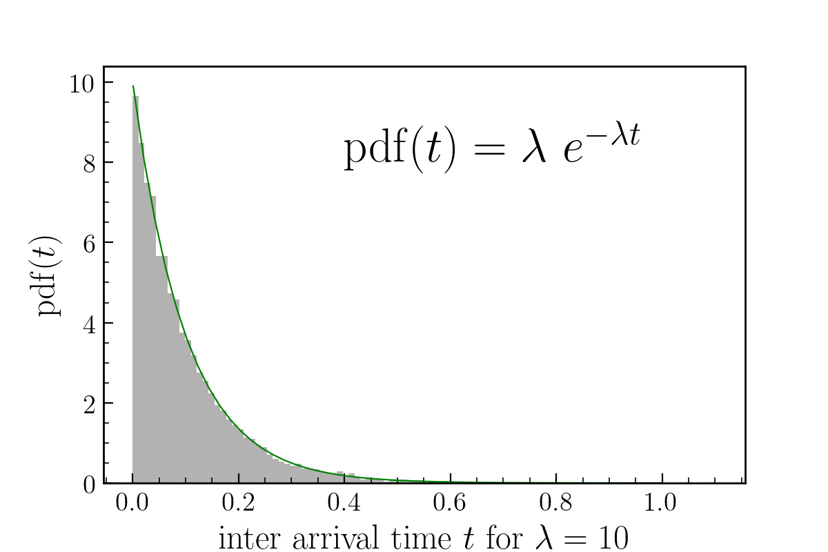
Now let’s say we were curious about counting the inter-arrival time between raindrops. Well if there are on average $\lambda$ drops falling per minute, the inter-arrival time on average should be $1/\lambda$. But what is the actual shape of the probability distribution of the inter-arrival times? In this case, the pdf is over a continuous domain and happens to be the exponential distribution. It has one free parameter and you guessed it, its the same $\lambda$ parameter that we have been using till now.
\[P(t|\lambda) = \lambda\ e^{-\lambda t}\ \forall\ t \ge 0\]

The distribution has mean $1/\lambda$ as we expected, and a variance of $1/\lambda^2$.
Here we can imaging a scenario. You decide to go inside to get your cup of tea. You now think how long will it take for you to see a raindrop on average once you go back outside. You calculate, on average the inter-arrival time is $1/\lambda = 6$ seconds. Given that you decide to go out randomly, it will take 3 seconds before you see the next raindrop. But is it?
Plotted are the arrival times(in seconds) of the first 20 drops that I simulated using $\lambda=10\ \mathrm{drops/min}$.

When you go out carrying your cup of tea which of the intervals(region between two drops) above are you more likely to hit. Obviously the regions with larger width. In other words, regions with larger width are oversampled. However these larger width regions also occurs less frequently (Refer fig. 2). So the probability distribution of encountering region $R$ of interval size $T$ is:
\[P(\mathrm{Region}\ R\ \mathrm{of\ size}\ T) = \lambda^2 T\ e^{-\lambda T}\]On expectation, the region that we are most likely to encounter has width given by:
\[E[W] = \int_0^\infty T\ pdf(T)\ dT = \int_0^\infty T\ \lambda^2 T\ e^{-\lambda T} = \frac{2}{\lambda}\]Since we are walking in randomly, the interval that we would observe is then half of the above value. But guess what this value is $1 / \lambda$, the expected arrival times between two raindrops, which in our case is 6 seconds and not 3 seconds are we thought before.
A take on this interesting phenomenon in case of bus arrival times, known as the waiting time paradox; which states:
When waiting for a bus that comes on average every 10 minutes, your average waiting time will be 10 minutes.
A nice discussion on this paradox can be found in this post by Jake Vanderplas. The waiting time paradox is a specific example of the inspection paradox.
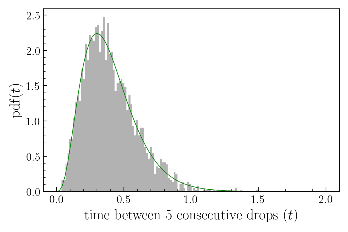
Let’s continue on our journey of exploring distributions via raindrops. You now ask, what is the time interval between $n$ consecutive raindrops? There are $n-1$ intervals between $n$ consecutive raindrops, with each interval having a size $t$ given by the exponential distribution. So what we want is the random variable which is the sum of $k = n-1$ exponentially distributed random variables. The pdf of this random variable is the Gamma distribution:
\[P(x | k, \lambda) = \frac{\lambda^k\ x^{k - 1} e^{-\lambda x}}{\Gamma(k)}\]

Our exploration uncovers a key finding that the various distributions are interconnected. For more such relations refer to this link. What we discussed was Poisson process in the time domain, raindrops or photons hitting a telescope; one can also have Poisson processes in the spatial domain. Its easier to visualize this in 2D, and we can take an example of trees growing in a forest. Analogous to the time domain discussion above, we have a rate parameter $\lambda$ which is number of trees per unit area. If we take a square of area A, move it across the forest, each time counting the number of trees that fall in the square, the count is going to be a random variable which, the same as before, is going to be Poisson distributed:
\[P(k\ \mathrm{trees\ in\ area}\ A) = \frac{ (\lambda A)^k e^{-\lambda A}}{k!}\]