``The Calculus required continuity, and continuity was supposed to require the infinitely little; but nobody could discover what the infinitely little might be."-- Bertrand Russell in Mysticism and Logic and Other Essays, The Floating Press, 1 August 2010, p.100
Many-a-time when working with model fitting to data, one encounters a situation where one need to find the probability distribution of a random variable, which itself is a function of another random variable.
Given that $x$ has a probability distribution $pdf_X(x)$, and that the variable $y$ is related to $x$ as $y = f(x)$, what is the probability distribution function of $y$?
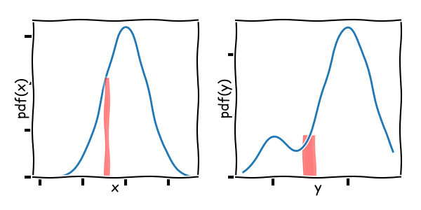
Naively, one might think for a given value $y’$, one can just pick up its probability as $f_X(x’)$, where $y’ = f(x’)$. This is correct when $x$ is a discrete random variable and we are talking about probability mass function. However, when $x$ is a continuous random variable, this approach gives wrong results. For the continuous case, the probability of a single point has no meaning. Rather, it is the probability of finding something in a given interval that is conserved across transformations. Making the interval become infinitesimal, we can approximate the area under the curve by a rectangle as shown in the figure. This area (mass) is the same when we transform to the variable $y$. In other words the following equality holds:
\[\mathrm{pdf}_X(x)\ dx = \mathrm{pdf}_Y(y)\ dy, \qquad ......dy = f'(x)\ dx\]
Let’s look at a few examples:
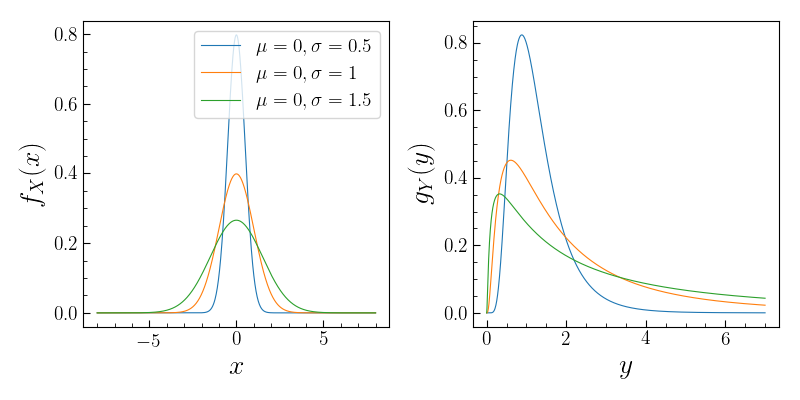
1. LogNormal Distribution: If $x$ is Gaussian distributed, then $y = e^x$ is said to have lognormal distribution. Let’s find its pdf using the above relation.
\[g_Y(y) = f_X(x) \frac{dx}{dy} = \frac{1}{\sqrt{2 \pi \sigma^2}} e^{-\displaystyle \frac{(x -\mu)^2}{2 \sigma^2}} \left(\frac{1}{y}\right) = \frac{1}{\sqrt{2 \pi \sigma^2}y} e^{-\displaystyle \frac{(\ln y -\mu)^2}{2 \sigma^2}}\]
2. Flux transmission: The flux field we observe from the absorption of Lyman-alpha photons by neutral Hydrogen in the intergalactic medium is related to the density field which is Gaussian in nature through the relation:
\[F(\mathbf{x}) = \exp \left[-A \exp \left(\beta \left[\delta_g(\mathbf{x}) - \frac{\sigma_g^2}{2} \right] \right) \right]\]The dependence of flux on density is thus highly non-linear. However, at earlier times when the variance on $\delta$ was small, the flux was roughly Gaussian distributed too. To find the exact pdf, we start by noting that:
\[\frac{dF}{d\delta_g} = \beta\ F \ln F\]Thus we have,
\[p(F) = -\frac{p(\delta_g)}{\beta\ F\ ln F},\]where $\delta_g$ for a given $F$ can be calculated from the first equation. We need a negative sign cause $F$ is a monotonically decreasing function of $\delta_g$.