One of the most common test case in supervised machine learning is that of classification: Given a data point, classify it into one of the many labels available
The simplest case of this is binary classification. For e.g. classifying emails as spam or ham, classifying objects as star or galaxy, classifying images as a cat or a dog, etc. In all these cases, to be able to apply the mathematical modeling of machine learning one needs to abstract away some feature(s) of the object. Most often choosing or engineering the right features is what gives more power to predictive modeling rather than sophisticated models.
If your features are crappy, no amount of sophisticated models can come to the rescue.
However, in this post we are going to assume that we already have the features in hand. Given this, there are broadly two different ways of approaching classification problems - parametric and non-parametric. The topic we are going to discuss falls in the non-parametric approaches; more specifically as a linear model.
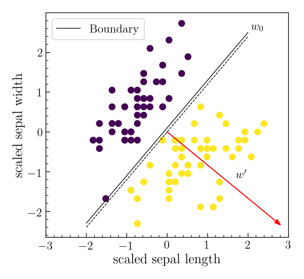
Logistic regression aims to creates a linear boundary separating objects of one class from the other. If the input features live in a $\mathcal{R}^d$ dimensional space, we want to create a $\mathcal{R}^{d-1}$ hyperplane optimally separating the two classes. The predicted class for any new point can then be inferred depending on which side of the hyperplane it lies. We will refer to this hyperplane as boundry.
\[y = sign(w^T x + b), \qquad y \in \{0, 1\}.\]We will take the class with label 1 as the positive class.
Conceptually, one can also think of the boundry as a set of points in the feature space whose probability of belonging to class $y=1$ is half. As we move away from the boundry, on one side the probability of belonging to $y=1$ diminishes, while on the other end it approaches 1.

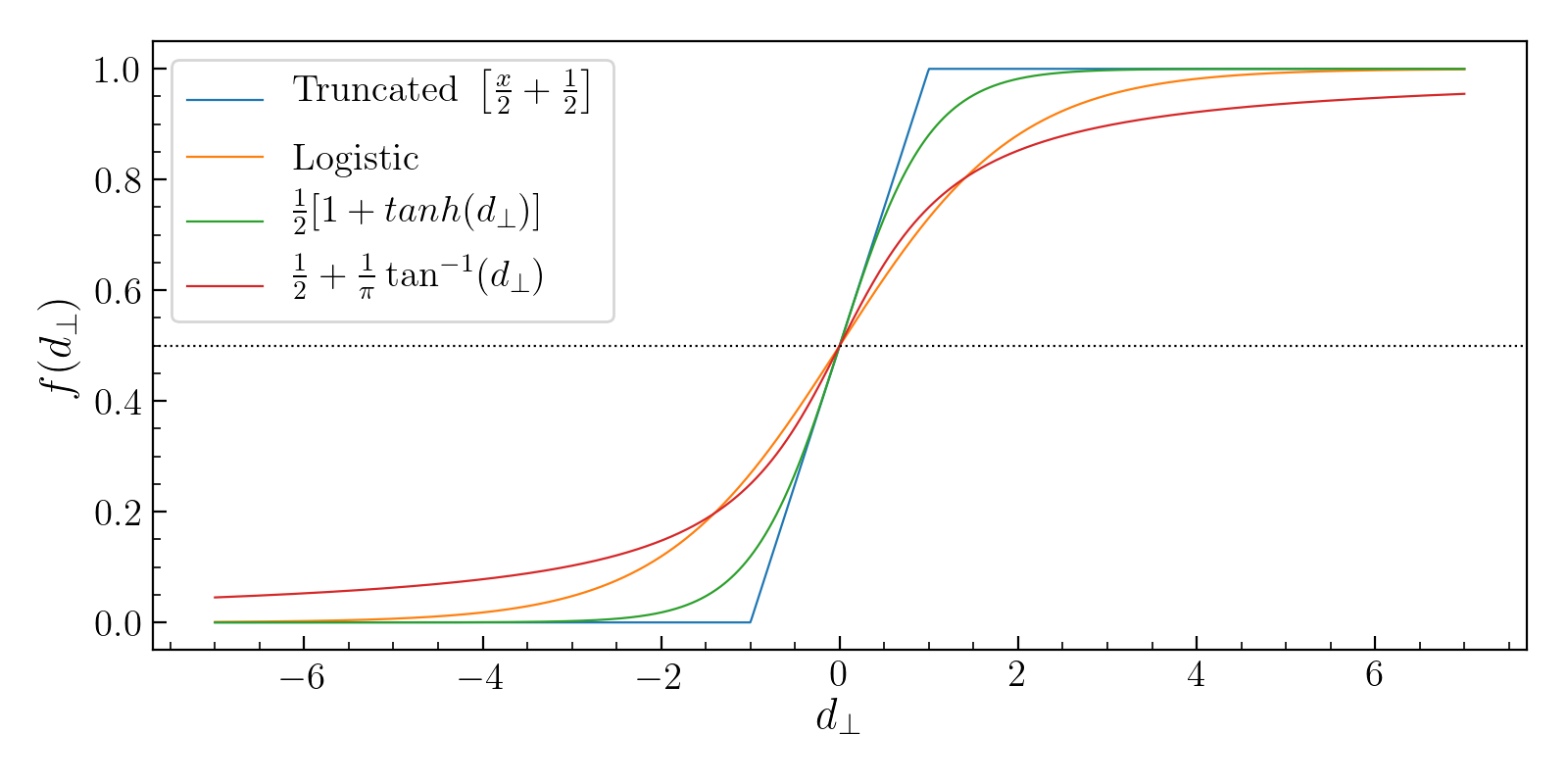
$\rightarrow$ Mathematically, what we want is a specific function of the perpendicular distance of any point from the boundary given by $z= w^Tx + b$, whose value on the boundary be 0.5 and should range from 0 to 1 as we move from one side of the boundary to the other.
There are many such functions that we could choose as shown below:

The functional form used by Logistic regression is the sigmoid function:
\[P(y=1|x) = \hat{y} = \sigma (z) = \frac{1}{1 + e^{-z}}\]One common terminology used in this regards is that of Odds. It is defined as:
\[\mathrm{Odds} = \frac{P(y = 1)}{P(y = 0)} = \frac{\hat{y}}{1 - \hat{y}}\]The domain of Odds lies in the range $[0, \infty)$. The natural logarithm of the above quantity is called Log Odds which lies in the range $(-\infty, \infty)$. This can be shown to be
\[\mathrm{Log Odds} = w^T x + b\]Thus we can interpret coefficient corresponding to a given predicting variable as: the change in log odds for a unit change in a given variable keeping the rest variables fixed.
$\rightarrow$ LogOdds = perpendicular distance; and the value of LogOdds on the boundary is 0.
Our goal in now to estimate the value of the parameters of the model, $w$, from training data. However, to assess which values of the parameters are good, we have to first define the likelihood. Under the assumption that each data-point is independent of every other data-point, we have:
\[\mathcal{L} = \prod_{i=1}^n p(y_i | x_i, w) = \prod_{i=1}^n [\mathcal{I}(y_i=1)\ \hat{y_i}][\mathcal{I}(y_i=0) (1 - \hat{y_i})]\]Remember, $\hat{y_i}$ gives the probability of a datapoint $i$ belonging to class $y=1$. So if a data-point belongs to $y=0$ we need to use $1 - \hat{y_i}$. Here $\mathcal{I}$ is an indicator variable to denote if a particular datapoint belongs to positive class or not. Writing in terms of log-likelihood and knowing that log of multiplication is equal to sum of the logs, this becomes:
\[\begin{align} \log\ \mathcal{L} &= \sum_{i=1}^n \left[\log[\mathcal{I}(y_i=1) \hat{y_i}] + \log [\mathcal{I}(y_i=0) (1 - \hat{y_i})] \right] \\ &= \sum_{i=1}^n \left[y_i \log \hat{y_i} + (1-y_i)\log (1 - \hat{y_i}) \right] \end{align}\]The value of $w$ we are looking for them becomes:
\[w_{ML} = \underset{w}{\mathrm{argmax}} (\log\ \mathcal{L})\]$\rightarrow$ One can also transform the likelihood to a cost function by simply taking the negative and reducing it via the mean, $C = -\frac{1}{n} \log \mathcal{L}$; hence the name negative-log-likelihood loss.
\[w_{ML} = \underset{w}{\mathrm{argmin}}\ C\]However, there is no analytical solution for $w$ given the form of the cost function. That’s where gradient descent comes to the rescue. We first randomly initialize $w$ and iteratively update it till a convergence criterion is reached.
\[w_{t+1} = w_t - \eta\ \nabla_w C,\]where $\eta$ is the learning rate.
The gradient of the cost function wrt $w$ can be obtained via chain rule:
\[\frac{dC}{dw} = -\frac{1}{n} \sum_{i=1}^n \frac{d \log \mathcal{L}_i}{dw} = -\frac{1}{n} \sum_{i=1}^n \left[ \frac{d \log \mathcal{L}_i}{d\hat{y_i}} \frac{d\hat{y_i}}{dz_i} \frac{dz_i}{dw}\right]\]The individual components in the chain can be written as:
\[\frac{dz_i}{dw} = \frac{d (w^T x_i + b)}{dw} = x_i\] \[\frac{d\hat{y_i}}{dz_i} = \frac{e^{-z_i}}{(1 + e^{-z_i})^2} = \hat{y_i} (1 - \hat{y_i})\] \[\frac{d \log \mathcal{L}_i}{d\hat{y_i}} = \frac{y_i}{\hat{y_i}} - \frac{(1-y_i)}{(1 - \hat{y_i})}\]Putting it all together, the gradient of the cost function wrt $w$ becomes:
\[\nabla_w\ C = -\frac{1}{n} \sum_{i=1}^n x_i [y_i (1 - \hat{y_i}) - (1 - y_i) \hat{y_i})] = -\frac{1}{n} \sum_i^n y_i x_i \left[\frac{1}{1 + e^{y_i w^T x_i}}\right].\]Likewise, the gradient of the cost function wrt the bias term $b$ can be written as:
\[\nabla_b\ C = -\frac{1}{n} \sum_i^n y_i \left[\frac{1}{1 + e^{y_i w^T x_i}}\right]\]More often that not, using the maximum likelihood prescription as above leads to estimates that have high variance. Especially in the case when one has fewer data-points than that is representative of the population, the classifier will be able to clearly separate the two classes with a linear boundary, with no misclassified points. In that case the value of $w$ will blow up. Points on either side of the boundary will be classified as belonging to their respective classes with probability of 1. This however may not generalize to new data-points and lead to a classifier with high variance. You basically read too much into your data, leading to overfitting.
This can be prevented using regularization. To keep the estimated $w$ from becoming too large, one can add a penalty term to the likelihood.
\[w_{reg} = \underset{w}{\mathrm{argmax}} \log\ \mathcal{L} - \lambda ||w||^2 \qquad \mathrm{Ridge}\] \[w_{reg} = \underset{w}{\mathrm{argmax}} \log\ \mathcal{L} - \lambda ||w||_1 \qquad \mathrm{Lasso}\]